Velocity, Force and the Jacobian
vω=q˙r=0
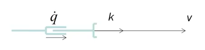
- q˙ is the rate of change of the joint position. (e.g., 0.5 m/s)
- k is the unit vector along the axis of translation. The direction of the movement/actuation.
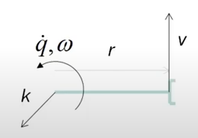
vω=q˙k×r=q˙k
- v is the velocity at the tool point.
- ω is the angular velocity of the tool point.
- q˙ is rotation speed. (e.g., 2 rad/s)
- k is the unit vector along the axis of rotation. z-axis
- r is the length of the link.
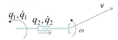
With more than one joint. tool point velocity components are a function of joint velocity and position.
[vω]=f(q˙1,q˙2,q1,q2)
- q˙ is the rotation speed of the joint.
- q is the joint position.
The Jocobian is a matrix that is a function of joint position, that linearly relates joint velocity to tool point velocity.
[vω]=J(q1,q2)[q˙1q˙2]
To compute the joint velocities for a given tool point velocity, we need to invert the Jacobian.
[vω]q˙=J(q)q˙=J−1(q)[vω]
The inverse Jocobian can be found by inverting a square portion of the Jacobian.
Find the joint velocities (q˙1,q˙2) in terms of the tool point velocity (x˙,y˙).
The arm points in the x direction, with joint 2 extended to 0.5 m. Find the joint velocities to move the tool point such that:
x˙=1m/sy˙=1m/s
[q˙1q˙2][q˙1q˙2]=−q21[sin(q1)−q2cos(q1)−cos(q1)−q2sin(q1)][x˙y˙]=−q21[0−0.5−10][11]=[21]
q˙_1q˙_2=2rad/s;=1m/s;
A singularity occurs when the Jacobian is not invertible. This happens when the determinant of the Jacobian is zero.
In the previous example, q2˙q˙1. If q˙2=0, then the Jacobian is not invertible. There are no valid joint velocity solutions.