Regularization
Regularization is a strategy used to build better-performing models by reducing the odds of overfitting, or when your model does such a good job of matching your training data that it performs badly on new data. In other words, regularization is a way to help your model generalize better by preventing it from becoming too complex.
Reduce the magnitude and/or the number of parameters to reduce model complexity.
One way to regularize a linear regression is to add a constraint to the loss function:
is a hyperparameter that controls the influence of our penalty.
Regularization seeks to penalize complex models
- A small change in input should lead to a small change in output value.
- Model complexity often leads to overfitting.
There are three main types of constraints: Ridge (L2), Lasso (L1), and Elastic Net.
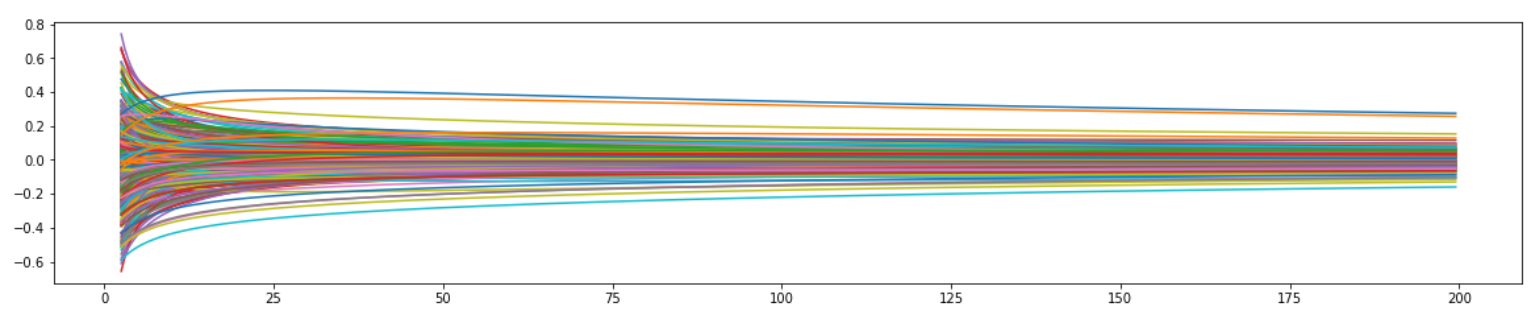
Ridge Regression (L2)
Ridge regression is also called L2 regularization. It adds a constraint that is the sum of the squared coefficients.
The second term is also known as shrinkage penalty.
- , this penalty term has no effect and ridge regression produces the same coefficients as least squares.
- As , the shrinkage penalty becomes more influential, the coefficients will approach 0.
Trace Plot
Python
Use sklearn's Ridge Regression.
from sklearn.linear_model import Ridge
import numpy as np
n_samples, n_features = 10, 5
rng = np.random.RandomState(0)
y = rng.randn(n_samples)
X = rng.randn(n_samples, n_features)
clf = Ridge(alpha=100.0) # alpha controls the strength of the penalty
clf.fit(X, y)
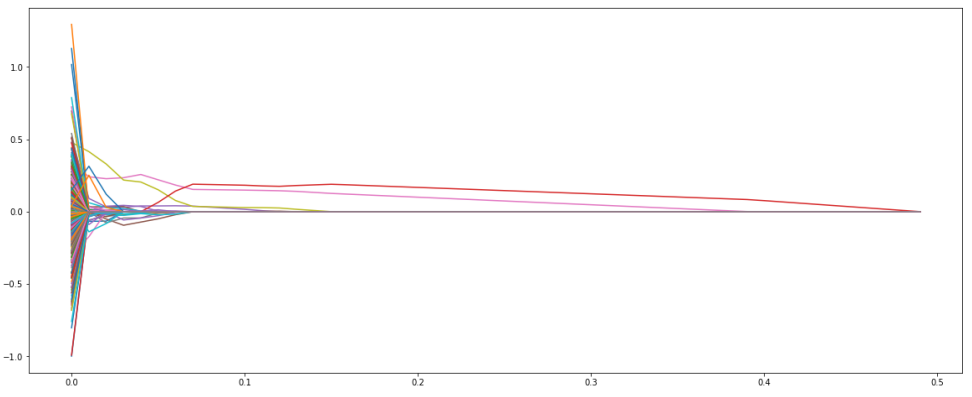
Lasso Regression (L1)
Lasso regression is also called L1 regularization. It also adds a constraint that is the sum of absolute coefficients.
It forces some of the coefficients to be zero and results a simpler model. Therefore it can be used to perform feature selection.
Trace Plot
Python
Use sklearn's Lasso Regression.
from sklearn.linear_model import Lasso
clf = Lasso(alpha=0.1) # alpha controls the strength of the penalty
clf.fit(X = [
                [0, 0],
                [1, 1],
                [2, 2]
            ],

        y = [0, 1, 2])

print(clf.coef_)

print(clf.intercept_)
Elastic Net
Elastic Net is the combination of the L1 regularization and L2 regularization. It can both shrink the coefficients as well as eliminate some of the insignificant coefficients.
Standardization
The values are transformed so their mean is 0, and their standard deviation is 1.
def standardize(data):
  """ Standardize/Normalize data to have zero mean and unit variance

  Args:
    data (np.array):
      data we want to standardize

    Returns:
      Standardized data, mean of data, standard deviation of data
  """
  mu = np.mean(data, axis=0) # rows - top to bottom
  sigma = np.std(data, axis=0) # rows - top to bottom
  scaled = (data - mu) / sigma
  return scaled, mu, sigma
Why standardization?
- For a given dataset, dimensions are usually in different scales. With regularization penalty, some dimensions might be penalized heavier than other dimensions.
- Easier to visualize.