Simple Linear Regression

Definition

Often we want to find a relationship between two variables to:

• Predict behavior
• Explore relationships

The simplest way to achieve this is to assume a linear relationship

info

Assumptions:

• Predictors are independent (not correlated)
• Residuals form a gaussian/normal distribution (bell curve)

On a qq-plot, that means they should form a straight line, for a histogram it means we should see a normal (bell) curve.

# plot qq-plot
statsmodels.api.qqplot(model.resid)
print(model.resid)

# plot histogram
fig = plt.figure(figsize=[8, 8])
ax = fig.add_subplot(1, 1, 1)
ax.hist(model.resid, 20)

$$y = \beta_0 +\beta_{1}x$$

offset + coefficient x variable

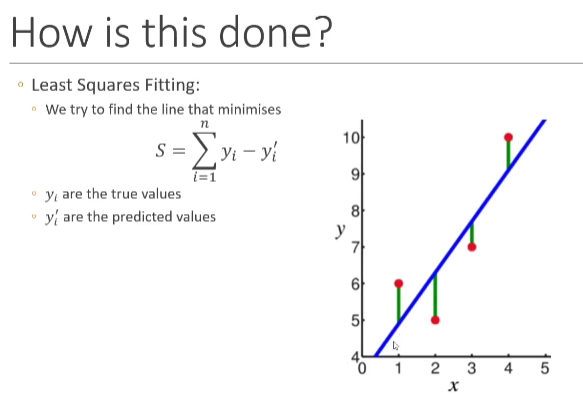
Minimize the Error

Try my best to estimate $\beta_0$ and $\beta_1$ given a set of observations, $y = (y_1,\ldots,y_n)$ and $x=(x_1,\ldots,x_n)$, so they can give the best $y$ given $x$

warning

In practice, our data is rarely on a straight line

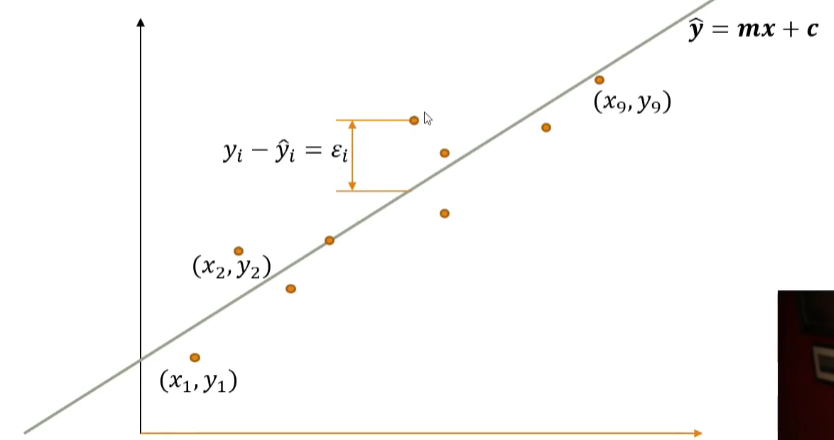
Point $i$ in our regression line is given by

$$y_i = mx_i + c +\epsilon_i$$

$\hat{y_i}$ is the predicted value, $y_i$ is the ground truth (observed) value. The difference between $\hat{y_i}$ and $y_i$ is called the error (residual) ~ $\epsilon_i$. We assume the residual is normally distributed around 0

The goal is to find the values of $c$ and $m$ that minimize the sum of the square of the errors

$$\sum^n_{i=1}\epsilon_i^2=\sum^n_{i=1}(y_i-\hat{y_i})^2=\sum^n_{i=1}(y_i - (mx_i + c))^2$$

note

Minimum requirement: the number of training samples should be much larger than the number of terms we are trying to estimate.

Correlation

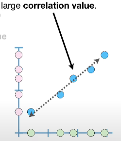
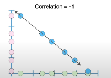
Definition: It describes the degree (ranges from -1 ~ 1) that two variables move in coordination with one another. If two variables move in the same direction, then those variables are said to have a positive correlation. If they move in opposite directions, then they have a negative correlation. It controls the strength and direction of the relationship.

$$Covariance = \frac{\sum (x- \bar{x})(y - \bar{y})}{n-1}$$

$$Correlation = \frac{Covariance(x, y)}{\sqrt{Variance(x)\sqrt{Variance(y)}}}$$

We can quantify the strength of the relationship with correlation. The sign (+/-) represents the direction of the relationship.

• -1, as one value increases the other decreases
• 0, no linear relationship, statically independent. It can still have other types of relationship.
• +1, increase and decrease together

note

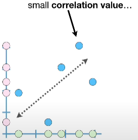
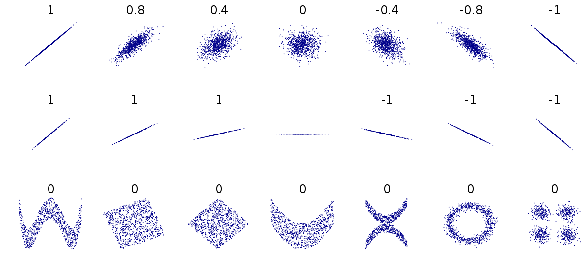
When the relationship cannot be represented with a straight line (linear relationship), correlation = 0.

danger

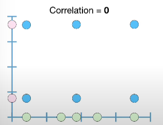
The correlation of a horizontal line is undefined. Because the variance is undefined or 0.

video sources:

1. Covariance - a computational step stone for calculating correlation.
2. Correlation

covariance

Why Do We Care?

1. If there is a linear relationship, we want to make sure the x is correlated with the result y.
2. Want our predictors to be uncorrelated with each other, since each predictor models a different aspect of the overall relationship. If they are correlated, we can end up with redundancy in the model.

Why do we want our predictors to be uncorrelated with each other?

In the "number of cyclists" case study, one of the linear regression model contains temp, and atemp as parameters, they are correlated, and thus the relationship between that variable and the response is (to some extent) captured twice in the model. That causes the p-value to be less important.